2 Numerical study

2.1 Normalized distance

In this paper, we are mainly interested in the horizontal distance traveled by the projectile. We first need to determine the angle α_s for which y as defined by Eq. (9) vanishes. This can be made by using the Newton-Raphson method with the initial value α_s = -α₀, corresponding to the solution in the absence of drag force. Therefore we compute

(10)

until |α_k+1 - α_k| reaches a value below a threshold, for example 0.01°. Once α_s is determined, we compute d = x(α_s) - x₀ using Eq. (9), which is the horizontal distance.

From Eq. (10), we can see that α_s only depends on α₀ and the ratio v₀∕v_lim. We will now denote this last quantity the normalized velocity v_norm. In the same way, if we normalize d by the distance traveled in the absence of drag force, defined as

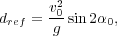(11)

then d_norm = d∕d_ref is only a function of α₀ and v_norm, and it can be computed independently from the drag coefficient λ. Consequently, we obtain a general result, which can be used for the study of the influence of different parameters for any kind of objects and drag coefficients. The normalized distance is drawn on Fig. 2

We see here the importance of using normalized quantities. From an initial problem featuring many parameters like the initial velocity v₀, the terminal velocity v_lim, the drag coefficient λ, the mass m, the launch angle α₀, and the distance d, we have derived a result in which they have been all wrapped in only three terms, namely the normalized distance, the normalized velocity, and the launch angle.

2.2 Parametrization

In order to easily study and use d_norm, we need to parametrize it, i.e. find an optimal set of parameters and functions that can fit its shape.

For α₀ fixed, we tried to describe d_norm as a function of v_norm using a Gaussian profile or a Lorentz profile, but the agreement was rather poor. We then tried using a Pearson VII function, which is an approximation of a Voigt profile:

(12)

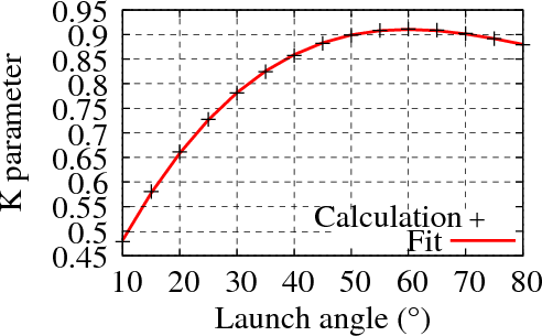
For M = 1, this reduces to a Lorentz profile, and for M →∞, it is a Gaussian profile (see annex A). The agreement is very good, as it can be seen on Fig. 3 for α₀ = 45°.

Parameters K and M are functions of α₀, their respective variations are plotted on Figs. 4 and 5.

They can easily be fitted using polynomials P_N(α₀) = ∑ _i=0^i=Na _iα₀ⁱ of degrees 3 and 2, which coefficients a_i are given in table 1.

Using coefficients of table 1 and Eq. (12), we managed to retrieve values calculated for Fig. 2 with a relative error lower than 0.2%. We can thus consider that the calculation of the horizontal traveled distance has been considerably simplified by comparison with the initial problem, whose solution required the numerical evaluation of Eq. (9) after Eq. (10) was solved. Respective influences of v₀, v_lim and α_O can now be studied without difficulty.

2.3 Example of application

We are interested in the influence of the launch angle on the horizontal distance. In the absence of drag force, the distance is given by Eq. (11), its maximum is achived for α₀ = 45°, and the distance traveled will be the same for α₀ = 45°±φ, with 0 < φ < 45°. If we take the drag force into account, the distance will no longer be symmetric with respect to α₀ = 45°, and a rapid observation of Fig. 2 tends to show that the distance will be greater for angles below 45°, what we may also intuitively think. Nevertheless, it should be noted that launch angles leading to the longest distance may be greater than 45° in some cases [8].

In the present case, using the work of section 2.2, we can easily compute d for a fixed v₀ by varying α₀, then search for which value α_O d reaches its maximum. This particular value of α₀ will be called the optimal launch angle. We perform our computation for a baseball [1, 5, 6] with λ∕m = 0.005376 m-1, i.e. v_lim = 42.7 m⋅s-1 and v₀ = v_norm.v_lim. Results are presented on Fig. 6.

This confirm that as v₀ increases, the optimal launch angle decreases.

The shape of the curve encourages us to once again try a fit with a Pearson function: α_max = h^-M. We set h = 45°, and the optimisation of the two others parameters leads to K = 0.0085864 s⋅m-1 and M = 0.1366571, which gives a maximal relative error smaller than 0.08% ! The choice of this function is thus validated.

As a last point, it should be stressed that using normalized quantities for solving physical problems sould not lead to overlook real quantities limits. In Sec. 1, it was pointed out that the domain of validity for the quadratic drag force hypothesis was dependant on the Reynolds number Re. For a baseball, we found that the velocity should not exceed 53 m⋅s-1, hence points calculated above this limit were grayed out on Fig. 6. The fact that they are well fitted using the previoulsy described Pearson function does not enforce in any way an extension of the domain of validity for the quadratic drag force hypothesis.