
We now intend to look more precisely at the case where the term l sin θ can no longer be neglected. For this sake, we propose two solutions: an approximate one, whose accuracy will be checked thanks to the second solution, which is analytical, thus exact, but practically unsuited.
We use a first order expansion of tan θ and sin θ, and by writing θ = θ0 + δθ we get
Using (3), (5) and (6) we obtain
 | (7) |
and we finally deduce the expression for δθ:
 | (8) |
Using this equation is only possible if Eqs. (5) and (6) are valid approximations, which means that δθ should be small enough, that is if l is small compared R. But how small it has to be before the error becomes too big is still unknown. Therefore, we need to know the real solution in order to evaluate the precision of Eq. (8).
By setting t = tan  , we can write sin θ =
  and tan θ =
  . Consequently, Eq. (3)
can be recasted as
. Consequently, Eq. (3)
can be recasted as
 | (9) |
and after simplification
 | (10) |
We now simply need to find a root of the previous equation between 0 and 1 in order to find θ (indeed, θ varies from 0 to π∕2, thus t varies from 0 to 1). Such a root exists, as P(0) < 0 and P(1) > 0, and it is unique. Moreover, it has an analytical expression, as it can be easily verified using computer algebra systems (the free software maxima for example), but the length and the complexity of this expression makes it unusable for practical purpose. Therefore, it is better to stick with a numerical evaluation of the root, by means of one of the many methods available (we used the methods implemented in the free software Octave).
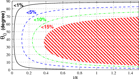
It is now possible to evaluate the relative error made on the solution θ when only the 0th-order solution is considered. This relative error is depicted on Fig. 2, where five zones are delimited, corresponding respectively to relative errors smaller than 1%, 5%, 10%, 15%, and bigger than 15%. Roughly, for l∕R < 0.1, the relative error is always smaller than 5%, and for l∕R < 0.4 it is always smaller than 15%.
Moreover, as previously announced, we can now also check the accuracy of the solution proposed in section 3.1. The relative error made on the solution θ when it is approximated by θ0 + δθ is shown on Fig. 3. The same zones as in the previous figure are drawn. It appears now that for l∕R < 0.2, the error is smaller than 1%, but for l∕R < 0.7, the error is still smaller than 10%, which is quite unexpected. Thus Eq. (8), despite its a priori limited range of validity, greatly enhances the basic solution given by Eq. (4).
 made on the determination of
 made on the determination of